In my last two posts, I described the techniques we used to create and enhance an ML data set for supervised learning. In my next post, we finally get to the really fun stuff – building models. But before I go there, I want to talk a little bit about the way we aggregated the data and the variables we created for the training. There are times when the raw data you have is the raw data you need for supervised ML learning. But in our case, we needed to tie the various tag signal strength readings together and, since we were aggregating multiple probes, we had to make decisions about how represent the data when aggregated.

 

As a quick reminder, our base raw data looks like this:

Tag is the sensor #, seq is a probe identifier, devsig is the device identifier, pwr is the Received Signal Strength on that sensor and tt is the Timestamp (store down to the milliseconds). The goal of the aggregation process was to create a single record that captured the signal strengths on every sensor for a given device.

 

In some cases, we aggregated by probe sequence so that only one signal could possible be received. But we also tried scenarios where we combined multiple probes together in a fixed time window. The time window was defined by two parameters: the total maximum time between the first signal and the last signal included, and the maximum allowable gap between signals. Typical values we tested were things like a time window of 1 second and a maximum gap of 400 milliseconds.

 

When we were aggregating by time window, we often had multiple signals on a single sensor. So we had to decide how to represent the power on that sensor. Initial exploratory analysis suggested that in most cases the signal strengths in a time window were nearly identical. But we were extra cautious about this and pretty much threw the kitchen sink at the problem. Our data set included the maximum power received, the minimum power received, the average power received, the median value and the modal value. Given our initial analysis, we weren’t exactly shocked that in most cases it didn’t make much difference which we used!

 

In the end, Avg. and Max tended to be the variables we ended up using – but in 9 cases out of 10 model performance was nearly identical across every representation.

 

Oh well…

 

For a store with eight sensors deployed (they all have more – I’m just lazy), you can think about our basic ML training observation looking like this:

 

Time

Device

Sensor 1 Reading (Avg. Signal Strength)

Sensor 2 Reading (Avg. Signal Strength)

Sensor 3 Reading (Avg. Signal Strength)

Sensor 4 Reading (Avg. Signal Strength)

Sensor 5 Reading (Avg. Signal Strength)

Sensor 6 Reading (Avg. Signal Strength)

Sensor 7 Reading (Avg. Signal Strength)

Sensor 8 Reading (Avg. Signal Strength)

 

But you know what, when you’re aggregating data this way you also have a count of how many signals each sensor detected in the window. This “PingCount” was included and turned out be more interesting than any of the statistical variants. It turns out that getting 6 probe signals on a sensor is a LOT more meaningful than getting 1.

 

Naturally, though, not every sensor will pick up a signal. So every observation had missing values. Missing values are a pain. We had three choices about how to handle this, and naturally we tried them all. One method was just to represent missing values as a very low signal strength. An RSSI value of something like -100. Since the lowest values we ever see are in the 90s, this would generally equate to a tag not picking up a signal. The second alternative was to categorize the signal strengths with one category being “No Signal”. That’s a perfect representation but categorizing the data for received signals is inevitably a little bit lossy. The third alternative was to structure the data so that the Tag and Signal were both values in the data set – only tags with values were represented. So we had a variable set like this:

 

Highest Tag: Tag1

Highest Tag Power: -48

Second Tag: Tag4

Second Tag Power: -53

Etc.

 

With this representation, you don’t have any missing values. In general, we discard observations with fewer than 3 sensor values. And in this last iteration, we tried models with three tag powers, four tag powers and five tag powers.

 

Each of these approaches worked reasonably well, but the first approach generally performed the best and was the easiest so most of the store models ended up using some variant of that approach.

 

Another way we tried to milk more value out of the data was with a concept called sensor pairs. The idea behind sensor pairs is that for determining an X or Y axis value, the difference between sensors aligned on that axis is particularly useful.

 

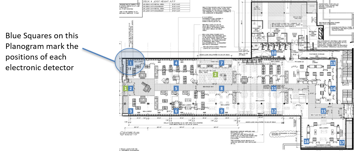
For sensor pairs, we’d identify which set of pairs had the highest reading. For the X-Axis was it 1,4,7,10,13 or 2,5,8,11,14 or 3,6,9,12,15 or 16,17. The group that had the highest power readings was then used to create power differences by subtracting the reading of sensors in each position (for example, the value at sensor 4 minus the value at sensor 1.

 

This turned out to be valuable both in some of the regressor models and some of the out-of-bounds models.

 

We tried a bunch of other things too, but in the end, the data set structure we generally looked kind of like this:

 

Device

TimeStamp

Calibration Point X,Y

Calibration Section

Calibration InBounds Flag

Sensor #1-#x Reading -Max RSI

Sensor #1-#x Reading-Min RSI

Sensor #1-#x Reading-Avg RSI

Sensor #1-#x Reading-RSI Mode

Sensor #1-#x Reading RSI Median

Sensor #1-#x Reading Ping Count

SensorPair #1-#x Differences

Count of Sensors with Signal (PingCount)

 

That’s pretty much it. Armed with this data set, we were ready to do some supervised learning.