There’s a rich history around the idea of data augmentation for Machine Learning. If you have a library of images you want to train a model on, you can use simple image manipulation techniques to create new rows of data. For images, this is really easy. You can flip, scale, rotate, crop or apply filters to images to create new but significantly different versions. You might, for example, change a filter on an image to create a series of images that reflect how the picture would look taken in different levels of light. That’s a powerful technique for creating good additional training data in cases where you have a supervised training set (like ours) that’s far smaller than the actual data you’re collecting.

 

Our training set is built from a small set of phones given to a calibrator who walks the floor for a significant amount of time. In some respects, our data is quite representative. It’s the same type of device shopper use and the same kind of signal we detect. Our calibrator places phones in various locations (hand, pocket, backpack) to simulate different carry heights and blockage patterns. But there are aspects of the process that are a little bit different than real-world data.

 

We realized this when we compared some key statistics from a calibration against similarly aggregated data from shoppers at the same location.

 

It probably requires a little bit of description for each metric to understand the meaning. When we get raw data from the sensors, we get a series of rows that look like this:

In this case, there are four sensors that saw a signal from the device in a probe cycle. When we turn this into an ML observation, all of these data points are aggregated into a single row with the power from each sensor reported. It’s actually more complicated than this since well often combine data from multiple probes that very close together, but that’s not important for this discussion. What’s important to understand is that these base rows get transformed into something like this:

 

Observation Time: 1/3/2019 22:14:19

# of Tags: 4

Highest Sensor: -50

Avg Sensor1: -73

Avg Sensor2: -65

Avg Sensor3: -60

Avg Sensor4: -50

 

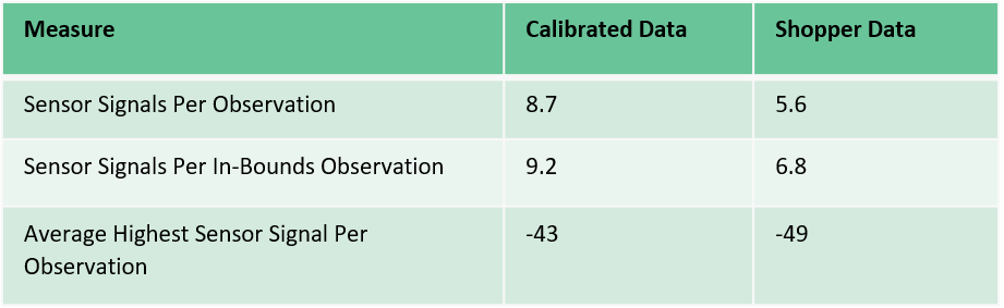
If a store has 20 sensors, it’s not unusual for 5 or 10 or even more to pick-up a signal.

 

In the table above, we’re looking at how many sensors– on average – picked up a signal. You can see that it’s much higher in our calibrated data – 8.7 sensors detected a signal per observation – compared to our overall shopper data – 5.6 sensors detected a signal per observation.

 

This was a red-flag for us when we looked at our data. It means that our calibration data is quite a bit richer than the average real-world observation – which isn’t going to make for a great model.

 

It was important for us to understand what was happening here and we did a deep dive into the data. We aggregate those probes into a set of values (you’ll see this later when I write about Model Building) and we generate all sorts of statistical representations including the Maximum Power Detected, Minimum Power Detected, Average Power, Modal Power and Median Power. We tried all of those variants and we also tried de-aggregating the sequences down to the lowest probe level so that we never had more than a single signal per probe.

 

What we found  is that our calibrating phones were cycling multiple times inside the time window that worked best for non-calibration aggregation. In other words, our continuous cycling was generating more data than a typical phone impacting all three of the variables above. With more signals, more sensors picked them up. And it was likelier that a close-by sensor wouldn’t miss a signal (more on that later). The probe rate is, of course, tune able in the App, but we found we could also adjust the time window for aggregating a probe and group the data using multiple time windows.

 

To make a long story short, we ended up aggregating the data in three different time windows. One – the long window – matched what we were doing with real shopper data. Then there was a medium window and a short window. The medium and short windows reported fewer sensors per observation (obviously)  and including them gave us a wider range of observations from which to train.

 

Adding the additional time windows didn’t quite triple the number of observations (shorter windows didn’t always find enough sensors to fingerprint from), but they more than doubled the total. And when we compared the same metrics from above, we’d moved much, much closer to matching our real-world data:

 

 

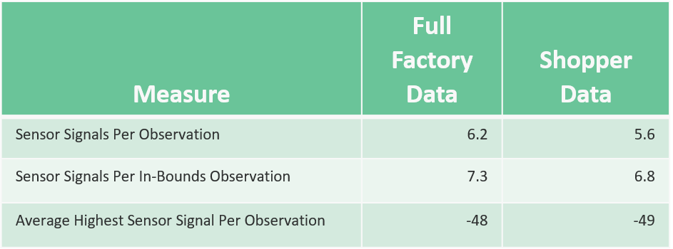
Using multiple time windows brought our calibration data set into very close alignment with our real shopper data. And it significantly improved model performance – especially in terms of the coherence of our different models in classifying real data.

 

This method worked pretty well but as we did more calibrations and tested more stores, we found we had a troubling problem with model outliers. The models worked very well for most signals but when strung together into visits they often showed single anomalous records.

 

When we extracted the observations that produced those records and ran them against the final models, we verified that the results were indeed weird and awful. Careful inspection of the data revealed that our models went seriously wrong when a sensor that was probably very close to a signal didn’t pick it up at all.

 

Imagine, for example, that Sensors #3, #4, #6 and #8 picked up signals, but Sensor #5 didn’t:

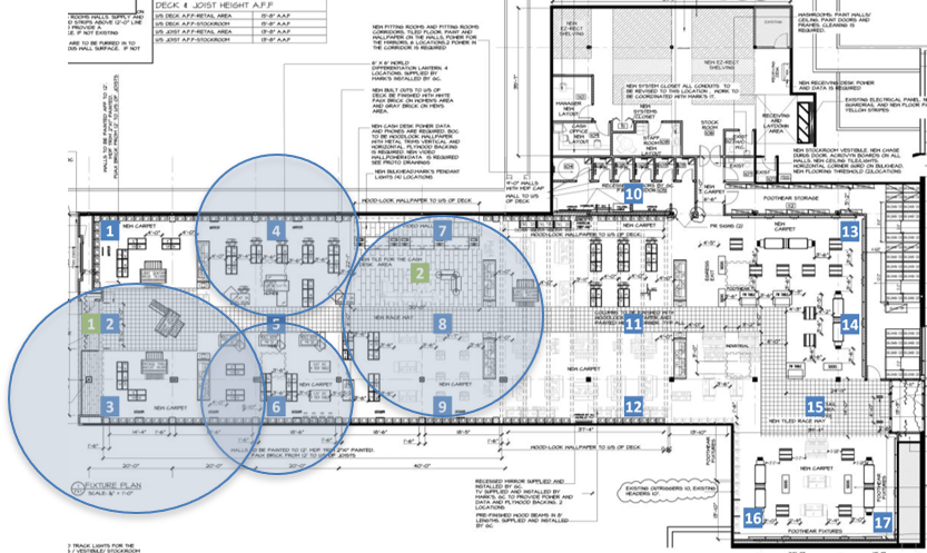
That’s a confusing situation and it shouldn’t happen. But it does. And it happens particularly often when the store is crowded and sensors get very busy. From our perspective, it looks like the system is prone to dropping the occasional sensor value when it gets heavily used. That ain’t great, of course, but it’s also outside our control since we’re not the hardware guys.

 

Our models weren’t handling this well – and since we did calibrations when the store was empty or uncrowded, it made sense. Our training data didn’t capture these situations because they didn’t occur much when you’re just calibrating.

 

To fix this, we added a data factory that took observations and sometimes duplicated them with one sensor value changed to missing. Because we usually pick up six or seven sensors, there’s plenty of data to support positioning even without any single tag. And by creating these extra records, we were able to make the ML less sensitive to the problems in hardware data collection.

 

Getting the data factory (sort of) right took a lot of work, a lot of study, and careful attention to the ways our training data could be transformed to match real-world circumstances better. You can’t randomly create data. And the potential to get this wrong and make things worse is very real.

 

But our situation isn’t all that uncommon. Limited training data is a common barrier to implementing ML processes. Some types of data – like images – are remarkably easy to transform and propagate (not that you don’t have to be careful there too). But careful attention to the ways your data might be interestingly transformed can make it possible to significantly increase the amount of valid ML training data you have.

 

And better training data means better ML.